I. Introduction to Benford's Law
Select any transaction from a typical general ledger. What are the odds that the dollar amount of the transaction begins with a 1? What are the odds that it begins with 2? How about 3? Or 9? Of the possible leading digits 1 through 9, one might assume that each has an equal 11.1% likelihood to be the first digit of a given transaction. However, this is actually incredibly unlikely (and if I observed this distribution of first digits across my general ledger I would be very concerned!).
In his 1938 paper, The Law of Anomalous Numbers, electrical engineer and physicist Frank Benford analyzed 20 unrelated sets of numbers collected from various sources and verified the expected frequencies of leading digits in a list of numbers. According to this analysis, the first digit of a given number is most likely to be 1, with a 30.1% probability, and least likely to be 9, at a 4.6% probability. This logarithmic distribution of leading digit frequencies is known as “Benford’s Law.” Benford also established equations for predicting the frequency of a given digit at a given position in a number, which we will be using in our implementation later in this article.
For example, the formula:
results in the following first digit probabilities for a data set that conforms to Benford’s Law:
| digit | probability |
|---|---|
| 1 | 30.1% |
| 2 | 17.6% |
| 3 | 12.5% |
| 4 | 9.7% |
| 5 | 7.9% |
| 6 | 6.7% |
| 7 | 5.8% |
| 8 | 5.1% |
| 9 | 4.6% |
By extension, the formula:
provides the expected Benford’s Law distribution for each possible combination of the first two digits of a number. Once again, the Benford’s Law distribution is quite different from a naive approach that assumes an equal 1.11% (1 / 90) chance of observing each first two leading digit combination.
| first two digits | probability |
|---|---|
| 10 | 4.1% |
| 11 | 3.8% |
| 12 | 3.5% |
| 13 | 3.2% |
| 14 | 3% |
| 15 | 2.8% |
| 16 | 2.6% |
| ... | ... |
| 99 | 0.44% |
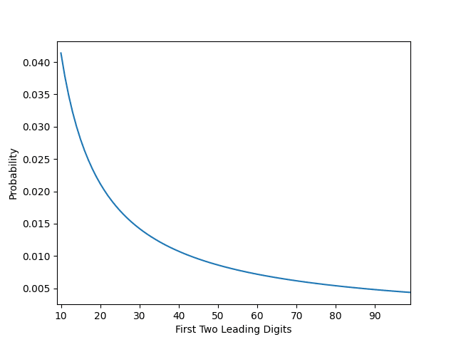
When analyzing Benford’s Law, it is useful to visualize the expected distribution for comparison against the observed distribution. Plotting the complete data from table above results in the line graph shown below, representing the expected frequency of each first two digit combination from 10 to 99. We will use this later.

Not all data sets will conform to Benford’s Law, but those that do are more likely to exhibit certain characteristics:
-
The data represents a sequence. For example, the Fibonacci sequence and a sequence of factorials both closely conform to Benford’s Law.
-
The data represents a combination of numbers from different distributions. For example, Benford’s analysis showed that the first digits of numbers extracted from a newspaper conformed to the expected frequencies. A newspaper article discussing stock prices would belong to one distribution, an article discussing home prices in the same newspaper belongs to another distribution, sports statistics represent a third distribution, etc.
-
The data spans several orders of magnitude.
-
The data is not confined to an upper or lower limit. For example, a list of adult human heights will not conform to Benford’s Law because in this case height has established boundaries. No one is 10 feet tall.
-
Data conforming to Benford’s Law is often described as “real”, “natural”, “scientific”, "measured”, etc. Invented or otherwise artificial numbers do not normally conform to Benford’s Law.
II. Benford’s Law and Accounting Data
The basic application of Benford’s Law to accounting data goes something like this:
A set of accounting data should not contain made-up numbers. If we have reason to expect that the data conforms to Benford’s Law, then non-conformity to the law is an indication that made-up numbers exist within the system. Investigation of this non-conformity could reveal fraud, waste, process inefficiency, or policy failures, among other things that an executive might want to know.
Before applying Benford’s Law to accounting data, it’s important to establish why we expect the data to conform to the law in the first place. Later in this article we will be testing two accounting datasets for conformity to Benford’s Law.
The first set is 2002 -2021 expenditures as reported by California cities in the City Financial Transaction Report maintained by the California State Controller’s Office, which is available to the public here. This data should conform to Benford’s Law because year-over-year expenditures represent a mathematical sequence whereby expenditures are multiplied by a somewhat consistent growth ratio. The varying size of each city should also ensure that the data spans several orders of magnitude.
The second set is Washington D.C. purchasing card data across the 2023 calendar year. This data is available to the public here. If this data represents a wide variety of different expense types, then we can assume that each expense type belongs to a different distribution. Data representing numbers from a combination of different distributions should conform to Benford's Law, as mentioned above.
III. First Two Digits Testing using Python
The following program takes a raw csv dataset to be tested against the expected Benford’s Law first two digit frequencies, compares the actual distribution to the expected distribution, and creates a dataframe that can be exported to excel or csv format for further analysis.
The program relies on numpy and pandas. I’m also using several functions defined in a separate utils file that are imported here.
import pandas as pd
import numpy as np
from utils import extract_first_digits, create_missing_values, create_graph
First, we want to create an array of the 90 possible first two leading digit combinations from 10 to 99.
first_two_digits = np.arange(10, 100)Next, create an array of expected proportions for the leading digit combinations using the appropriate Benford’s Law formula.
benford_frequencies = np.log10(1 + (1 / first_two_digits))These two arrays are needed to calculate conformity to Benford’s Law and will eventually serve as columns of our report output.
Read the raw data into a pandas dataframe and use the “usecols” parameter to isolate the column containing the dollar amounts to be tested. In the California City Expenditures data, this column is named “Value.”
# file_name contains the file path to a source csv file.
purchases_df = pd.read_csv(file_name, usecols=["Value"])
Use the pandas map() method to apply the extract_first_digits() function that was imported earlier to each element in the dataframe. extract_first_digits() won’t act on numbers less than 10, resulting in empty entries for these numbers. We need to remove these entries from the resulting dataframe with the dropna() method. The size variable tracks the size of the new dataframe after dropping values less than 10.
purchases_df = purchases_df.map(extract_first_digits).dropna()
size = purchases_df.size
extract_first_digits() gathers the first two digits of each number by converting the number to a string and splicing string indexes 0 and 1. This operation is not very efficient for very large numbers, but should be good enough for our purposes.
def extract_first_digits(data):
    if data >= 10:
       return int(str(data)[:2])
Using the size variable from the previous step, we can create the next array that will be used in our output dataframe: the expected count of each leading digit combination according to Benford’s Law. This line creates a list of expected counts by multiplying each previously calculated expected proportion by the total size of our data set.
expected_counts = [i * size for i in benford_frequencies]Finally, we create arrays containing the actual count and actual leading digit proportions observed in our data. This can be done with the pandas value_counts() method and passing the parameter normalize=True for the proportions.
actual_counts = purchases_df["Value"].value_counts()
actual_proportions = purchases_df["Value"].value_counts(normalize=True)
While not it’s not likely, it’s theoretically possible that our data does not contain a particular leading digit combination in a smaller sample size. In this case, we want to make sure that the digit combination is still included in our analysis with a count and proportion of zero. The following block takes care of that using the imported create_missing_values() function.
def create_missing_values(full_set, partial_set):
    missing_digit_combinations = []

    for digits in full_set:
        if digits in partial_set.keys():
            continue
        else:
            missing_digit_combinations.append(digits)

    missing_fill = np.zeros(len(missing_digit_combinations))

    return pd.Series(missing_fill, missing_digit_combinations)
if actual_proportions.size < 90:
missing_proportions = create_missing_values(first_two_digits, actual_proportions)
missing_counts = create_missing_values(first_two_digits, actual_counts)
complete_actual_proportions = pd.concat([actual_proportions, missing_proportions]).sort_index()
complete_actual_counts = pd.concat([actual_counts, missing_counts]).sort_index()
d = {"FIRST_TWO_DIGITS": first_two_digits,
"EXPECTED_COUNTS": expected_counts,
"ACTUAL_COUNTS": complete_actual_counts,
"EXPECTED_FREQUENCIES": benford_frequencies,
"ACTUAL_FREQUENCIES": complete_actual_proportions}
else:
d = {"FIRST_TWO_DIGITS": first_two_digits,
"EXPECTED_COUNTS": expected_counts,
"ACTUAL_COUNTS": actual_counts.sort_index(),
"EXPECTED_FREQUENCIES": benford_frequencies,
"ACTUAL_FREQUENCIES": actual_proportions.sort_index()}Here we also take the output arrays created in the prior steps and add them to Python dictionary "d".
Next we create our output dataframe by instantiating a new pandas dataframe with the dictionary.
benford_df = pd.DataFrame(data=d)…but this doesn’t yet tell us anything about how well our data conformed to Benford’s Law. To do that we can take advantage of pandas’ element-wise operations to create two new columns calculating both the Z statistic and the absolute deviation between the observed and expected leading digit frequencies.
benford_df["ABSOLUTE_DEVIATION"] = (abs(benford_df["ACTUAL_FREQUENCIES"] - benford_df["EXPECTED_FREQUENCIES"]))
benford_df["Z_STATISTIC"] = ((abs(benford_df["ACTUAL_FREQUENCIES"] - benford_df["EXPECTED_FREQUENCIES"]) - (1 / (2 * size)))
                              / np.sqrt((benford_df["EXPECTED_FREQUENCIES"] * (1 - benford_df["EXPECTED_FREQUENCIES"])) / size ))
Calculate the mean absolute deviation using the absolute deviation column and pandas’ mean() method.
mean_absolute_deviation = benford_df["ABSOLUTE_DEVIATION"].mean()Finally, we can plot the results using the create_graph() function imported earlier. We'll also print the first five rows of the the final dataframe to confirm that it contains the information we want. As mentioned earlier, this dataframe can be exported to csv or excel for other users.
def create_graph(digits, expected, actual, mad, bar_color="silver", line_color="darkblue"):
    fig, ax = plt.subplots()
    bins = digits
    values = actual
    ax.bar(bins, values, color=bar_color, label="Actual Frequencies")
    ax.plot(digits, expected, color=line_color, label="Benford's Law Expectation")
    ax.legend()
    ax.text(x=55, y=0.035, s=f'MAD: {mad:.4f}')
    plt.xticks(np.arange(10, 91, 10))
    plt.xlim(left=9, right=99)
    plt.show()
return fig, axcreate_graph(benford_df["FIRST_TWO_DIGITS"],
benford_df["EXPECTED_FREQUENCIES"],
benford_df["ACTUAL_FREQUENCIES"],
mean_absolute_deviation)print(benford_df.head())IV. Running the code with real data
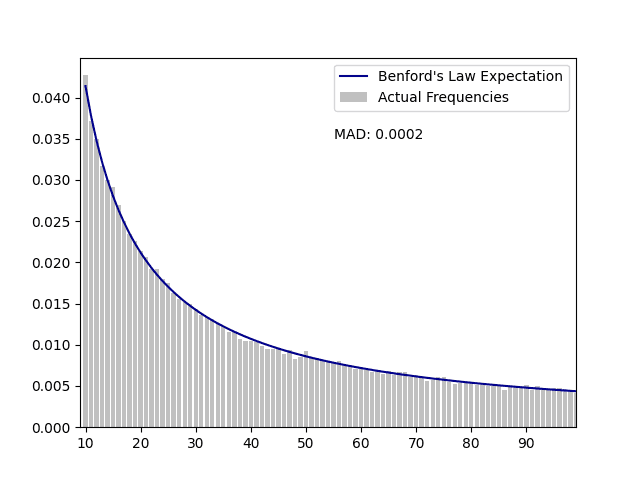
City Financial Transaction Report - with a mean absolute deviation of .0002, this data exhibits close conformity to Benford's Law.
Graph:

First five rows of the output:
    FIRST_TWO_DIGITS  EXPECTED_COUNTS  ACTUAL_COUNTS  EXPECTED_FREQUENCIES  ACTUAL_FREQUENCIES  ABSOLUTE_DEVIATION  Z_STATISTIC
              10      8712.208194           8990              0.041393            0.042713            0.001320     3.034258
              11      7953.622930           7811              0.037789            0.037111            0.000678     1.624600
              12      7316.623839           7349              0.034762            0.034916            0.000154     0.379309
              13      6774.135602           6677              0.032185            0.031723            0.000462     1.193477
              14      6306.569367           6322              0.029963            0.030037            0.000073     0.190892
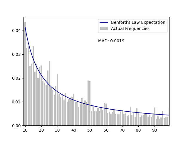
2023 Washington D.C. Purchasing Cards - while this data exhibits a general trend towards the Benford's Law curve, conformity to the curve is minimal. There are also numerous visible peaks and valleys in the graph.
Graph:

First five rows of the output:
    FIRST_TWO_DIGITS  EXPECTED_COUNTS  ACTUAL_COUNTS  EXPECTED_FREQUENCIES  ACTUAL_FREQUENCIES  ABSOLUTE_DEVIATION  Z_STATISTIC
              10      1639.688437           1725              0.041393            0.043546            0.002154     2.139213
              11      1496.918263           1289              0.037789            0.032540            0.005249     5.465283
              12      1377.031315           1317              0.034762            0.033247            0.001515     1.632888
              13      1274.931862            989              0.032185            0.024967            0.007218     8.125736
              14      1186.933168           1022              0.029963            0.025800            0.004164     4.845986
So, we've run an initial Benford's Law analysis on two sets of real world data. One shows close conformity to Benford's Law, while the other does not. Where do we go from here? Could the second data set have certain attributes that explain the deviations from Benford's Law? We'll explore that in a later post.